Cluster analysis or clustering is the task of grouping a set of objects in such a way that objects in the same group (called a cluster) are more similar (in some sense) to each other than to those in other groups (clusters). It is a main task of exploratory data analysis, and a common technique for statistical data analysis, used in many fields, including pattern recognition, image analysis, information retrieval, bioinformatics, data compression, computer graphics and machine learning.
Cluster analysis itself is not one specific algorithm, but the general task to be solved. It can be achieved by various algorithms that differ significantly in their understanding of what constitutes a cluster and how to efficiently find them. Popular notions of clusters include groups with small distances between cluster members, dense areas of the data space, intervals or particular statistical distributions. Clustering can therefore be formulated as a multi-objective optimization problem. The appropriate clustering algorithm and parameter settings (including parameters such as the distance function to use, a density threshold or the number of expected clusters) depend on the individual data set and intended use of the results. Cluster analysis as such is not an automatic task, but an iterative process of knowledge discovery or interactive multi-objective optimization that involves trial and failure. It is often necessary to modify data pre-processing and model parameters until the result achieves the desired properties.
Besides the term clustering, there are a number of terms with similar meanings, including automatic classification, numerical taxonomy, botryology (from Greek βότρυς “grape”), typological analysis, and community detection. The subtle differences are often in the use of the results: while in data mining, the resulting groups are the matter of interest, in automatic classification the resulting discriminative power is of interest.
Cluster analysis was originated in anthropology by Driver and Kroeber in 1932 and introduced to psychology by Joseph Zubin in 1938 and Robert Tryon in 1939 and famously used by Cattell beginning in 1943 for trait theory classification in personality psychology.
The notion of a “cluster” cannot be precisely defined, which is one of the reasons why there are so many clustering algorithms. There is a common denominator: a group of data objects. However, different researchers employ different cluster models, and for each of these cluster models again different algorithms can be given. The notion of a cluster, as found by different algorithms, varies significantly in its properties. Understanding these “cluster models” is key to understanding the differences between the various algorithms. Typical cluster models include:
- Connectivity models: for example, hierarchical clustering builds models based on distance connectivity.
- Centroid models: for example, the k-means algorithm represents each cluster by a single mean vector.
- Distribution models: clusters are modeled using statistical distributions, such as multivariate normal distributions used by the expectation-maximization algorithm.
- Density models: for example, DBSCAN and OPTICS defines clusters as connected dense regions in the data space.
- Subspace models: in biclustering (also known as co-clustering or two-mode-clustering), clusters are modeled with both cluster members and relevant attributes.
- Group models: some algorithms do not provide a refined model for their results and just provide the grouping information.
- Graph-based models: a clique, that is, a subset of nodes in a graph such that every two nodes in the subset are connected by an edge can be considered as a prototypical form of cluster. Relaxations of the complete connectivity requirement (a fraction of the edges can be missing) are known as quasi-cliques, as in the HCS clustering algorithm.
- Signed graph models: Every path in a signed graph has a sign from the product of the signs on the edges. Under the assumptions of balance theory, edges may change sign and result in a bifurcated graph. The weaker “clusterability axiom” (no cycle has exactly one negative edge) yields results with more than two clusters, or subgraphs with only positive edges.
- Neural models: the most well known unsupervised neural network is the self-organizing map and these models can usually be characterized as similar to one or more of the above models, and including subspace models when neural networks implement a form of Principal Component Analysis or Independent Component Analysis.
A “Clustering” is essentially a set of such clusters, usually containing all objects in the data set. Additionally, it may specify the relationship of the clusters to each other, for example, a hierarchy of clusters embedded in each other. Clusterings can be roughly distinguished as:
- Hard clustering: Each object belongs to a cluster or not
- Soft clustering (also: fuzzy clustering): Each object belongs to each cluster to a certain degree (for example, a likelihood of belonging to the cluster)
There are also finer distinctions possible, for example:
- Strict partitioning clustering: Each object belongs to exactly one cluster
- Strict partitioning clustering with outliers: Objects can also belong to no cluster, and are considered outliers
- Overlapping clustering (also: alternative clustering, multi-view clustering): Objects may belong to more than one cluster; usually involving hard clusters
- Hierarchical clustering: Objects that belong to a child cluster also belong to the parent cluster
- Subspace clustering: While an overlapping clustering, within a uniquely defined subspace, clusters are not expected to overlap
Applications of Clustering in different fields
- Marketing: It can be used to characterize & discover customer segments for marketing purposes.
- Biology: It can be used for classification among different species of plants and animals.
- Libraries: It is used in clustering different books on the basis of topics and information.
- Insurance: It is used to acknowledge the customers, their policies and identifying the frauds.
Hierarchical Clustering
In data mining and statistics, hierarchical clustering (also called hierarchical cluster analysis or HCA) is a method of cluster analysis which seeks to build a hierarchy of clusters.
Hierarchical clustering, also known as hierarchical cluster analysis, is an algorithm that groups similar objects into groups called clusters. The endpoint is a set of clusters, where each cluster is distinct from each other cluster, and the objects within each cluster are broadly similar to each other.
Strategies for hierarchical clustering generally fall into two types:
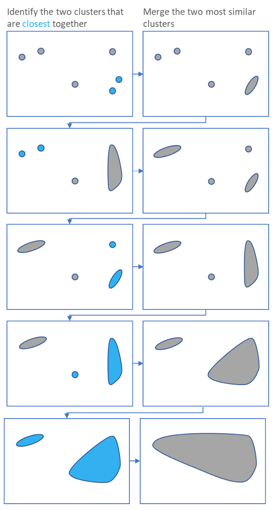
- Agglomerative: This is a “bottom-up” approach: each observation starts in its own cluster, and pairs of clusters are merged as one moves up the hierarchy.
- Divisive: This is a “top-down” approach: all observations start in one cluster, and splits are performed recursively as one moves down the hierarchy.
In general, the merges and splits are determined in a greedy manner. The results of hierarchical clustering are usually presented in a dendrogram.
Measures of distance (Similarity)
In the example above, the distance between two clusters has been computed based on the length of the straight line drawn from one cluster to another. This is commonly referred to as the Euclidean distance. Many other distance metrics have been developed.
The choice of distance metric should be made based on theoretical concerns from the domain of study. That is, a distance metric needs to define similarity in a way that is sensible for the field of study. For example, if clustering crime sites in a city, city block distance may be appropriate. Or, better yet, the time taken to travel between each location. Where there is no theoretical justification for an alternative, the Euclidean should generally be preferred, as it is usually the appropriate measure of distance in the physical world.
Linkage Criteria
After selecting a distance metric, it is necessary to determine from where distance is computed. For example, it can be computed between the two most similar parts of a cluster (single-linkage), the two least similar bits of a cluster (complete-linkage), the center of the clusters (mean or average-linkage), or some other criterion. Many linkage criteria have been developed.
As with distance metrics, the choice of linkage criteria should be made based on theoretical considerations from the domain of application. A key theoretical issue is what causes variation. For example, in archeology, we expect variation to occur through innovation and natural resources, so working out if two groups of artifacts are similar may make sense based on identifying the most similar members of the cluster.
Where there are no clear theoretical justifications for the choice of linkage criteria, Ward’s method is the sensible default. This method works out which observations to group based on reducing the sum of squared distances of each observation from the average observation in a cluster. This is often appropriate as this concept of distance matches the standard assumptions of how to compute differences between groups in statistics (e.g., ANOVA, MANOVA).
Agglomerative versus divisive algorithms
Hierarchical clustering typically works by sequentially merging similar clusters, as shown above. This is known as agglomerative hierarchical clustering. In theory, it can also be done by initially grouping all the observations into one cluster, and then successively splitting these clusters. This is known as divisive hierarchical clustering. Divisive clustering is rarely done in practice.